VLOOKUP Function
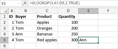
The VLOOKUP function is one of the lookup and reference functions. It is used to perform the vertical search for a value in the left-most column of a table or an array and return the value in the same row based on a specified column index number.
The VLOOKUP function syntax is:
VLOOKUP (lookup-value, table-array, col-index-num[, [range-lookup-flag]])
where
lookup-value is a value to search for.
table-array is two or more columns containing data sorted in ascending order.
col-index-num is a column number in the table-array, a numeric value greater than or equal to 1 but less than the number of columns in the table-array
range-lookup-flag is a logical value TRUE or FALSE. It is an optional argument. Enter FALSE to find an exact match. Enter TRUE or omit this argument to find an approximate match, in this case if there is not a value that strictly matches the lookup-value, then the function will choose the next largest value less than the lookup-value.
Note: if the range-lookup-flag is set to FALSE, but no exact match is found, then the function will return the #N/A error.
To apply the VLOOKUP function,
- select the cell where you wish to display the result,
- click the Insert function
 icon situated at the top toolbar,
or right-click within a selected cell and select the Insert Function option from the menu,
or click the icon situated at the formula bar,
- select the Lookup and Reference function group from the list,
- click the VLOOKUP function,
- enter the required arguments separating them by comma,
- press the Enter button.
The result will be displayed in the selected cell.
